Matrix Manipulations

MATLAB: The Language of Technical Computing

Hey folks!
Today's lesson is gonna go big! While the previous lesson was just on making simple matrices and performing simple operation over them, today's lesson is gonna go advanced.
Once a matrix is made, it needs to be manipulated. Learn how to concatenate, index, randomize, sort, shift, reshape/resize, rotate, flip matrices with proper code snippets!


Before everything, let us first learn how to write fundamental comments in MATLAB, just like other fundamental languages. To do so, we precede everything we are gonna add as comments with a percentage symbol ( % ).
Just like you can see here: 

Adding comments in MATLAB

Also, let us learn a new way to define matrices in MATLAB.

This method is used when we know the value that need to be entered in the matrix we want to generate and those values are of a type of set range. Just like if matrix needs to contain values from 1 to 5.

In this code snippet below you can see we have entered very generic values. Hence we defined the matrix in the above form.

Defining a matrix when a range of elements is used

In this way, A contains row #1 of 1 to 5, row #2 containing values from 6 to 10, #3 from 11 to 15, #4 from 16 to 20, #5 from 21 to 25. 

In very simple words, if the values are in a pre-defined range, we can write

A=[1:5];

Instead of

A=[1 2 3 4 5];

Having seen MATLAB on the simplest levels, lets move on towards achieving the objectives we outlined in the beginning of the post.
Hence the objectives for this post are as following:

Matrix Manipulations:

• Concatenating
• Indexing
• Randomization
• Sorting
• Shifting
• Reshaping & Resizing
• Rotation
• Flipping about a Vertical/Horizontal Axis

Hence lets move on towards achieving our objectives for today's post!

Matrix Manipulations

Concatenating

Just like in actual world, where concatenation is used to join smaller things to make something bigger, concatenation has the same application in MATLAB. Using concatenation we can join smaller matrices to produce bigger matrices. As in a matrix, its most fundamental unit is an element of that matrix, an entire matrix can be seen as an amalgamation of all the elements in your matrix. In other words, a matrix can be viewed as a product of concatenation of all the different elements of that matrix.

It is performed very simply in MATLAB. To concatenate two matrices, the following commands are implemented. Analyse them carefully.

A=[2,5,6;1,4,3;5,8,4];

B=[1,4,6;4,3,2;8,7,9];

C=[A;B];

display(A);

display(B);

display(C);

As you may note, the square brackets are used to bind both the matrices together inside a single matrix separated by a semi colon.

The above set of commands produce the following output. Closely observe the workspace window.

Concatenation of matrices

Indexing

Indexing on a matrix means selecting a subset of elements from itself. Indexing as a function is used as a first or primary operation before many advanced operations. There are many types of indexing possible as well, depending upon whether you want to select individual elements out of a given matrix or a set or range of elements. In this tutorial we would be learning 3 indexing methods primarily given as below:

• Selecting an individual element from a matrix
• Selecting a set of predefined elements from a matrix
• Selecting a set of unknown range of elements from a matrix

For indexing an individual element from a matrix, let us assume a matrix A we define below and let us assume we need to see index the 5th element from the same matrix. The commands for the same would be:

A=[1 2 3 4 5 6];
B=A(5);
display(A);
display(B);

The above commands hence produce an output as following:

Indexing of individual elements from a matrix

One important thing to notice while indexing individual elements from multidimensional matrices is that the indexing counter works in a column major order. In other words, if you suppose want to index an element at 4th position in the matrix, the counter will go along the columns and then find the 4th element and display that. You can see that for yourself here:

Indexing individual elements from multidimensional arrays

As you may see here, first when a 2x3 matrix was declared and it was asked to fetch the 4th element, the counter went along the first column first, oversaw element 1 and 2, then switched to the 2nd column, consisting element #3 and 4. Hence the 4th element was 5.
Again as we changed the order of the matrix, made it a 3x2 matrix, we found that the 4th element becomes 2. WHY? Because the counter now when goes along the first column, encounters element #1, 2 and 3. Then it switches to column #2 and hence the first element that it encounters is element #4. Hence 2 is the 4th element here.

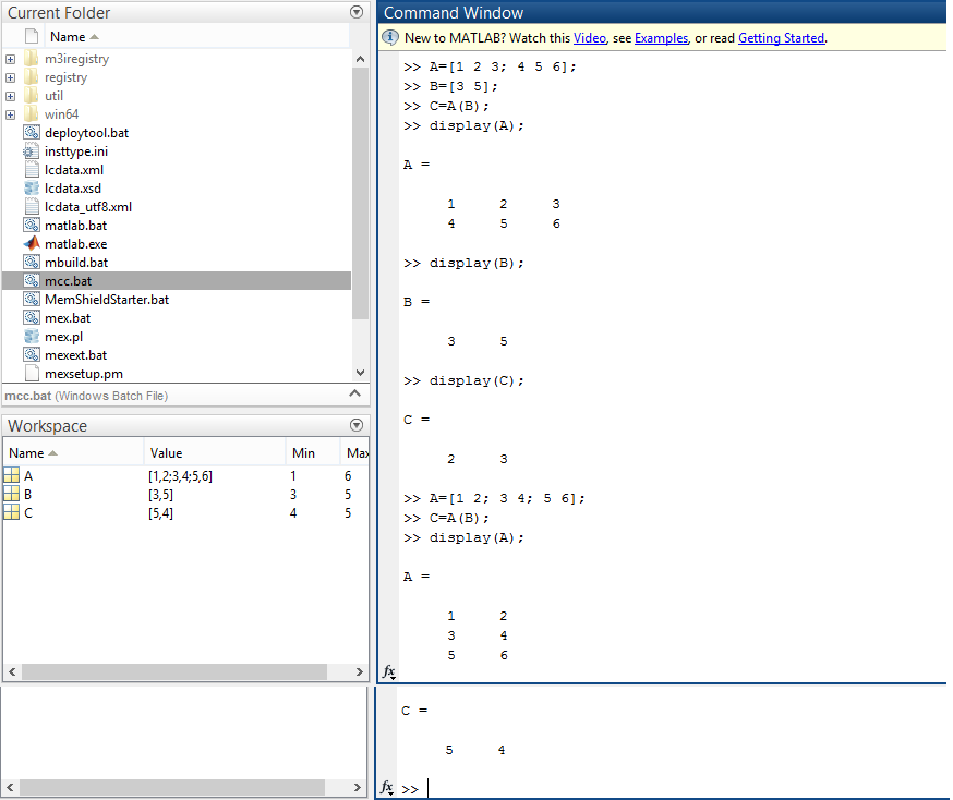
For indexing a set of predefined elements from a matrix, let us assume the same orders of 1D ( 1x6 ) and 2D ( 2x3 and 3x2 ) matrices we assumed above. Suppose we now wish to obtain the 3rd and 5th elements from those matrices. What we would do this time is combine the element numbers we wish to index as a single vector.
For example as we wish to obtain element #3 and #5, we would create B=[3 5]; And then we would use this matrix for our purpose of indexing. This can be seen as below:

A=[10 9 4 8 5 1];
B=[3 5];
C=A(B);
display(A);
display(B);
display(C);

The output hence produced is:

Indexing a predefined set of elements from a 1D Matrix

Similarly for a 2D matrix,

Indexing a set of predefined values from a 2D Matrix

For selecting a set of unknown range of elements from a matrix, we use a colon to separate the lower limit and upper limit of the range of elements we wish to index. For example, to select a range of elements ranging from the 2nd element to the 5th one, we would execute the following commands:

For a 1D matrix:

A=[1 2 3 4 5 6];

C=A(2:5);

display(A);

display(C);

which produces the output as shown.

Selecting a set of unknown elements from a 1D matrix

Similarly for a 2D matrix, the commands that need to be used are:

A=[1 2 3; 4 5 6];

C=A(2:5);

display(A);

display(C);

A=[1 2; 3 4; 5 6];

display(A);

display(C);

The above commands would produce the output:

Selecting a set of unknown elements from a 1D matrix

Randomization

MATLAB is in many ways similar to other major programming languages that you might have studied before. As another proof of that, MATLAB can be used to generate random matrices, just like there are implementations possible in other languages to generate random numbers.

To generate square random matrices in MATLAB, use the following commands:

A=rand(4);

display(A);

The above command will generate a square random matrix of 4x4 as below. The only argument that the rand() takes is the order of the random matrix you want to create, like 4 in this case.

Generating random matrices

To generate a random matrix of a variable order, you can use the same rand( m x n ) in the following manner:

A=rand(3, 2);
display(A);

This would create a random matrix of the order 3x2 as below:

Generating random matrices of variable order

Additionally, you might have noticed that the random numbers obtained are always positive. If we want to include negative numbers as well in our set of random numbers, we need to use a different function; randn(); It works just the same way as rand, whenever we want to display square random matrices or random matrices of a variable order. It can be seen as below:

Including negative random numbers using randn function

Sorting

Just like we operated while indexing matrices, in a column major order, sorting of matrices works in the same manner. To sort a matrix in ascending order, use the commands as below:

A=rand(3);

B=sort(A);

display(A);

display(B);

And this will produce the following output:

Sorting a matrix in ascending order

By default, the numbers are sorted in ascending order. The strings 'ascend' and 'descend' can be used to change the default order. To sort the same matrix in a descending order, we must enter commands as following:

A=rand(3);

B=sort(A, 'descend');

display(A);

display(B);

And the following output will be produced:

Shifting

Shifting of matrices takes place in term of rows and/or columns. MATLAB allows us to shift rows and/or columns simultaneously in individual commands. This leaves us with the following three instances in which we can shift rows and/or columns.

• Shifting individual rows
• Shifting individual columns
• Shifting rows and columns

I'd recommend learning each type above with the help of examples, as I feel that'd make the concepts clear in the first go itself. Hence lets continue.

Shifting Individual Rows. To shift individual rows, consider the following code:

A=[1:5; 6:10; 11:15; 16:20; 21:25];
B=circshift(A, [3,0]);
display(A);
display(B);

You might notice the use of command circshift(); This function is used to shift the rows or columns of a matrix. The shifting is done in a cyclic manner. The arguments given to the circshift function inside the parentheses determine 

• The matrix upon which shifting will be operated
• Whether the rows or columns or both will be operated

In the above commands the circshift function takes two arguments. The first argument given is the name of the matrix, A. Then we give the vector [3, 0] as a direction to cyclically shift the matrix A in a row major order, 3 rows in a cyclic order. The above command will hence cycle the first row 3 times in the cyclic order.

Shifting Individual Columns, similar to how we shift rows, to shift columns, enter the following code:

A=[1:5; 6:10; 11:15; 16:20; 21:25];
B=circshift(A, [0,3]);
display(A);
display(B);


Since the vector given as an argument to circshift() is [0,3], the matrix A will get cycled thrice cyclically in a column major order.

Shifting rows and columns simultaneously. By now I expect you to know the trick. To shift the rows and columns simultaneously, we do the following code.

A=[1:5; 6:10; 11:15; 16:20; 21:25];
B=circshift(A, [3,3]);
display(A);
display(B);

Since the vector given as an argument to circshift() is [3,3], the matrix A will get cycled thrice cyclically both in a row major and column major order.

The output produced in all the three cases would be as following:

Shifting of matrix rows and/ or columns in MATLAB

Reshaping and Resizing

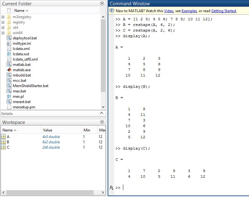
Reshaping a matrix means changing the order of the matrix. It is done when for example we create a matrix of the order (m x n) while we actually wanted it to be of the order (p x q) or just of any other order but (m x n).

Let us assume A to be a matrix of the order ( i , j ). To reshape the matrix to the order x, y. Such that number of elements in both matrices are same, use the command:

A = [1 2 3; 4 5 6; 7 8 9; 10 11 12];

B = reshape(A, 6, 2);

C = reshape(A, 2, 6);

display(A);

display(B);

display(C);

where the values of x and y are 6 and 2 respectively for matrix B. Similarly x and y have the values 2 and 6 for the matrix C.

So as we have seen, thee reshape function takes three arguments

• Name of the matrix to be reshaped
• New value of the number of rows in the new matrix
• New value of the number of columns in the new matrix

The output produced hence is as following:

Reshaping Matrices

Rotation

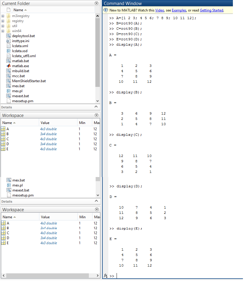
In MATLAB, we can rotate a matrix after we have it created. The rotation occurs in counter-clockwise direction. The default function, rot90 rotates a matrix in the counter clockwise direction for 90 degrees. However we can have a rotation at a multiple of 90 degrees using a different set of arguments than what rot90 takes. Let us see both the functions operating in the two examples below.

In the first example, we would create a matrix A and give it 4 rotations 90 degree each using the default rot90 function as below so that the final matrix obtained is a copy of the matrix we started with. The commands to be used are:

A=[1 2 3; 4 5 6; 7 8 9; 10 11 12];

B=rot90(A);

C=rot90(B);

D=rot90(C);

E=rot90(D);

display(A);

display(B);

display(C);

display(D);

display(E);

Using default arguments with rot90 function

In the second example, we rotate a given matrix directly to its initial orientation by giving the multiple of 90 the matrix is to be rotated at along with the matrix name in the argument list of rot90 function. The commands used are:

A=[1 2 3; 4 5 6; 7 8 9; 10 11 12];

B=rot90(A, 4);

display(A);

display(B);

The output produced is as following:

Using additional arguments with rot90 function in place of the default rot90 function

Flipping about a Vertical/Horizontal Axis

To understand flipping about axes, first we should be able to understand axes. In terms of MATLAB, up-down form the vertical axis while left-right form the horizontal axis. Hence to flip matrices, the following function is used

• To flip along the horizontal axis: fliplr(matrix name);
• To flip along the vertical axis: flipud(matrix name);

 The examples illustrating the same are as following: 

Flipping matrices

With that we finish out today's lesson. Though this was a long post, I'm sure we learnt a lot out of it. Stay tuned and take care! :)